Analyze with IMAS-Python
For this part of the training we will learn to open an IMAS database entry, and plot some basic data in it using matplotlib.
Open an IMAS database entry
IMAS explicitly separates the data on disk from the data in memory. To get
started we load an existing IMAS data file from disk. The on-disk file
is represented by an imas.DBEntry, which we have to
open() to get a reference to the data file we
will manipulate. The connection to the data file is kept intact until we
close() the file. Note that the on-disk file
will not be changed until an explicit put() or
put_slice() is called.
We load data in memory with the get() and
get_slice() methods, after which we
can use the data.
Hint
Use the ASCII data supplied with IMAS-Python for all exercises. It contains two
IDSs (equilibrium and core_profiles) filled with data from three
time slices of ITER reference data. A convenience method is available in the
imas.training module to open the DBEntry for this training data:
imas.training.get_training_db_entry() returns an opened
imas.DBEntry object.
Exercise 1
Open the training database entry: entry = imas.training.get_training_db_entry()
Load the
equilibriumIDS into memory using theentry.getmethodRead and print the
timearray of theequilibriumIDSLoad the
core_profilesIDS into memoryExplore the
core_profiles.profiles_1dproperty and try to match \(t\approx 433\,\mathrm{s}\) to one of the slices.Note
core_profiles.profiles_1dis time dependent with coordinatecore_profiles.time[1]. This means thatcore_profiles.profiles_1d[i]corresponds to the timecore_profiles.time[i].Read and print the 1D electron temperature profile (\(T_e\),
core_profiles.profiles_1d[i].electrons.temperature) from thecore_profilesIDS at time slice \(t\approx 433\,\mathrm{s}\)
import imas.training

# Open input data entry
entry = imas.training.get_training_db_entry()

# 1. Read and print the time of the equilibrium IDS for the whole scenario
#    This explicitly converts the data from the old DD version on disk, to the
#    new DD version of the environment that you have loaded!
equilibrium = entry.get("equilibrium")  # All time slices
# 2. Print the time array:
print(equilibrium.time)

# 3. Load the core_profiles IDS
core_profiles = entry.get("core_profiles")
# 4. When you inspect the core_profiles.time array, you'll find that item [1]
#    corresponds to t ~ 433s.
# 5. Print the electron temperature
print(core_profiles.profiles_1d[1].electrons.temperature)

# Close input data entry
entry.close()
Caution
When dealing with unknown data, you shouldn’t blindly get() all data:
large data files might quickly fill up the available memory of your machine.
The recommendations for larger data files are:
Only load the time slice(s) that you are interested in.
Alternatively, IMAS-Python allows to load data on-demand, see Lazy loading for more details.
Exercise 2
Write a function that finds the closest time slice index to
\(t=433\,\mathrm{s}\) inside the equilibrium IDS. Use the
equilibrium.time property
Hint
Create an array of the differences between the equilibrium.time
array and your search term (\(t=433\,\mathrm{s}\)).
Now the index of the closest time slice can be found with
numpy.argmin().
import numpy as np
import imas.training


# Find nearest value and index in an array
def find_nearest(a, a0):
    "Element in nd array `a` closest to the scalar value `a0`"
    idx = np.abs(a - a0).argmin()
    return a[idx], idx


# Open input data entry
entry = imas.training.get_training_db_entry()

# Read the time array from the equilibrium IDS
eq = entry.get("equilibrium")
time_array = eq.time

# Find the index of the desired time slice in the time array
t_closest, t_index = find_nearest(time_array, 433)
print("Time index = ", t_index)
print("Time value = ", t_closest)

# Close input data entry
entry.close()
Attention
IMAS-Python objects mostly behave the same way as numpy arrays. However, in some cases
functions explicitly expect a pure numpy array and supplying an IMAS-Python object raises
an exception. When this is the case, the .value attribute can be used to obtain
the underlying data.
Note
IMAS-Python has two main ways of accessing IDSs. In the exercises above, we used the “attribute-like” access. This is the main way of navigating the IDS tree. However, IMAS-Python also provides a “dict-like” interface to access data, which might be more convenient in some cases. For example:
import imas.training

# Open input data entry
entry = imas.training.get_training_db_entry()

cp = entry.get("core_profiles")
for el in ["profiles_1d", "global_quantities", "code"]:
    print(cp[el])

# You can also get sub-elements by separating them with a '/':
print(cp["profiles_1d[0]/electrons/temperature"])
Retreiving part of an IDS
If the data structure is too large, several problems may pop up:
Loading the data from disk will take a long(er) time
The IDS data may not fit in the available memory
To overcome this, we can load only part of the IDS data from disk.
Retrieve a single time slice
When we are interested in quantities at a single time slice (or a low number of time
slices), we can decide to only load the data at specified times. This can be
accomplished with the aforementioned get_slice()
method.
Exercise 3
Use the get_slice() method to obtain the electron density
\(n_e\) at \(t\approx 433\,\mathrm{s}\).
Hint
get_slice() requires an interpolation_method as one
of its arguments, here you can use imas.ids_defs.CLOSEST_INTERP.
import imas.training

# Open input data entry
entry = imas.training.get_training_db_entry()

# Read n_e profile and the associated normalised toroidal flux coordinate at
t = 443  # seconds

cp = entry.get_slice("core_profiles", t, imas.ids_defs.CLOSEST_INTERP)

# profiles_1d should only contain the requested slice
assert len(cp.profiles_1d) == 1

ne = cp.profiles_1d[0].electrons.density
rho = cp.profiles_1d[0].grid.rho_tor_norm
print("ne =", ne)
print("rho =", rho)

# Close the datafile
entry.close()
Attention
When working with multiple IDSs such as equilibrium and core_profiles the
time arrays are not necessarily aligned. Always check this when working with random data!
Now we can plot the \(n_e\) profile obtained above:
Exercise 4
Using matplotlib, create a plot of \(n_e\) on the y-axis and
\(\rho_{tor, norm}\) on the x-axis at \(t=433\mathrm{s}\)
import os

import matplotlib
import imas.training

# To avoid possible display issues when Matplotlib uses a non-GUI backend
if "DISPLAY" not in os.environ:
    matplotlib.use("agg")
else:
    matplotlib.use("TKagg")

import matplotlib.pyplot as plt

# Open input data entry
entry = imas.training.get_training_db_entry()

# Read n_e profile and the associated normalised toroidal flux coordinate at
t = 443  # seconds

cp = entry.get_slice("core_profiles", t, imas.ids_defs.CLOSEST_INTERP)

# profiles_1d should only contain the requested slice
assert len(cp.profiles_1d) == 1

ne = cp.profiles_1d[0].electrons.density
rho = cp.profiles_1d[0].grid.rho_tor_norm

# Plot the figure
fig, ax = plt.subplots()
ax.plot(rho, ne)
ax.set_ylabel(r"$n_e$")
ax.set_xlabel(r"$\rho_{tor, norm}$")
ax.ticklabel_format(axis="y", scilimits=(-1, 1))
plt.show()
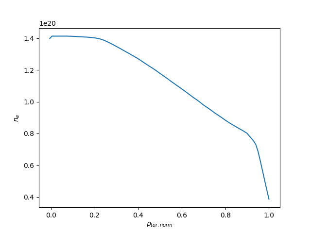
A plot of \(n_e\) vs \(\rho_{tor, norm}\).
Lazy loading
When you are interested in the time evolution of a quantity, using get_slice may be
impractical. It gets around the limitation of the data not fitting in memory, but will
still need to read all of the data from disk (just not at once).
IMAS-Python has a lazy loading mode, where it will only read the requested data from disk
when you try to access it. You can enable it by supplying lazy=True to a call to
get() or get_slice().
Exercise 5
Using matplotlib, create a plot of \(T_e[0]\) on the y-axis and
\(t\) on the x-axis.
Note
Lazy loading is not very useful for the small training data. When you are on the ITER cluster, you can load the following data entry with much more data, to better notice the difference that lazy loading can make:
import imas
from imas.ids_defs import MDSPLUS_BACKEND

database, pulse, run, user = "ITER", 134173, 106, "public"
data_entry = imas.DBEntry(MDSPLUS_BACKEND, database, pulse, run, user)
data_entry.open()
import os

import matplotlib
import numpy

# To avoid possible display issues when Matplotlib uses a non-GUI backend
if "DISPLAY" not in os.environ:
    matplotlib.use("agg")
else:
    matplotlib.use("TKagg")

from matplotlib import pyplot as plt

import imas
from imas.ids_defs import MDSPLUS_BACKEND

database, pulse, run, user = "ITER", 134173, 106, "public"
data_entry = imas.DBEntry(
    MDSPLUS_BACKEND, database, pulse, run, user, data_version="3"
)
data_entry.open()
# Enable lazy loading with `lazy=True`:
core_profiles = data_entry.get("core_profiles", lazy=True)

# No data has been read from the lowlevel backend yet
# The time array is loaded only when we access it on the following lines:
time = core_profiles.time
print(f"Time has {len(time)} elements, between {time[0]} and {time[-1]}")

# Find the electron temperature at rho=0 for all time slices
electon_temperature_0 = numpy.array(
    [p1d.electrons.temperature[0] for p1d in core_profiles.profiles_1d]
)

# Plot the figure
fig, ax = plt.subplots()
ax.plot(time, electon_temperature_0)
ax.set_ylabel("$T_e$")
ax.set_xlabel("$t$")
plt.show()
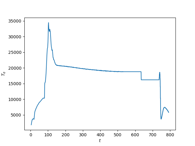
A plot of \(T_e\) vs \(t\).
See also
Explore the DBEntry and occurrences
You may not know a priori which types of IDSs are available within an IMAS database entry. It can also happen that several IDSs objects of the same type are stored within this entry, in that case each IDS is stored as a separate occurrence (occurrences are identified with an integer value, 0 being the default).
In IMAS-Python, the function list_all_occurrences() will
help you finding which occurrences are available in a given database entry and for a given
IDS type.
The following snippet shows how to list the available IDSs in a given database entry:
import imas

# Open input data entry
entry = imas.DBEntry("imas:hdf5?path=<...>", "r")

# Print the list of available IDSs with their occurrence
for idsname in imas.IDSFactory().ids_names():
    for occ in entry.list_all_occurrences(idsname):
        print(idsname, occ)

entry.close()